how to draw plane in 3d plot python

There are many problems in engineering that require examining a 2-D domain. For example, if you desire to decide the distance from a specific bespeak on a flat surface to any other flat surface, you need to think near both the x and y coordinate. At that place are various other functions that need ten and y coordinates.

Contents

  • 1 Introductory Links
  • 2 Individual Patches
    • 2.1 Trinket Version
  • 3 The meshgrid Command
  • 4 Examples Using 2 Independent Variables
  • 5 Examples Using Refined Grids
  • half dozen Using Other Coordinate Systems
  • seven Color Bars
  • 8 In that location Is No Endeavor
  • ix Questions
  • 10 External Links
  • eleven References

Introductory Links

To better sympathise how plotting works in Python, start with reading the post-obit pages from the Tutorials page:

  • Usage Guide
  • Pyplot tutorial
  • Image tutorial
  • The mplot3d Toolkit
  • 3D plotting examples gallery

Besides, there are several first-class tutorials out there! For example:

  • Three-Dimensional Plotting in Matplotlib from the Python Data Scientific discipline Handbook past Jake VanderPlas.

Individual Patches

One way to create a surface is to generate lists of the x, y, and z coordinates for each location of a patch. Python tin can brand a surface from the points specified by the matrices and will then connect those points by linking the values next to each other in the matrix. For example, if x, y, and z are 2x2 matrices, the surface will generate group of iv lines connecting the four points and and so fill in the space amongst the 4 lines:

                        import            numpy            as            np            from            mpl_toolkits.mplot3d            import            axes3d            import            matplotlib.pyplot            as            plt            fig            =            plt            .            figure            (            num            =            1            ,            clear            =            Truthful            )            ax            =            fig            .            add_subplot            (            i            ,            ane            ,            1            ,            projection            =            '3d'            )            ten            =            np            .            assortment            ([[            1            ,            3            ],            [            two            ,            4            ]])            y            =            np            .            assortment            ([[            v            ,            6            ],            [            7            ,            8            ]])            z            =            np            .            array            ([[            9            ,            12            ],            [            10            ,            eleven            ]])            ax            .            plot_surface            (            10            ,            y            ,            z            )            ax            .            set            (            xlabel            =            '10'            ,            ylabel            =            'y'            ,            zlabel            =            'z'            )            fig            .            tight_layout            ()            fig            .            savefig            (            'PatchExOrig_py.png'            )          

PatchExOrig py.png

Trinket Version

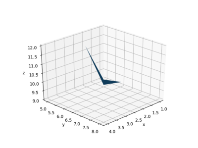
Note that the 4 "corners" in a higher place are not all co-planar; Python will thus create the patch using 2 triangles - to prove this more conspicuously, y'all can tell Python to change the view by specifying the elevation (angle up from the xy aeroplane) and azimuth (bending around the xy plane):

                        ax            .            view_init            (            elev            =            xxx            ,            azim            =            45            )            plt            .            describe            ()          

which yields the following paradigm:

PatchExRot py.png

You lot tin can add more than patches to the surface by increasing the size of the matrices. For example, calculation some other column will add together two more than intersections to the surface:

                        fig            =            plt            .            effigy            (            num            =            1            ,            clear            =            True            )            ax            =            fig            .            add_subplot            (            i            ,            1            ,            ane            ,            projection            =            '3d'            )            x            =            np            .            array            ([[            1            ,            3            ,            five            ],            [            two            ,            4            ,            6            ]])            y            =            np            .            assortment            ([[            5            ,            6            ,            5            ],            [            7            ,            8            ,            9            ]])            z            =            np            .            assortment            ([[            9            ,            12            ,            12            ],            [            10            ,            11            ,            12            ]])            ax            .            plot_surface            (            x            ,            y            ,            z            )            ax            .            set up            (            xlabel            =            'x'            ,            ylabel            =            'y'            ,            zlabel            =            'z'            )            ax            .            view_init            (            elev            =            30            ,            azim            =            220            )            fig            .            tight_layout            ()          

PatchExTwoRot py.png

Annotation the rotation to better see the two different patches.

The meshgrid Control

Much of the fourth dimension, rather than specifying private patches, y'all will have functions of two parameters to plot. Numpy's meshgrid control is specifically used to create matrices that will represent two parameters. For example, note the output to the post-obit Python commands:

                        In            [            one            ]:            (            x            ,            y            )            =            np            .            meshgrid            (            np            .            arange            (            -            ii            ,            two.1            ,            1            ),            np            .            arange            (            -            1            ,            1.1            ,            .            25            ))            In            [            2            ]:            ten            Out            [            2            ]:            array            ([[            -            2.            ,            -            1.            ,            0.            ,            ane.            ,            2.            ],            [            -            2.            ,            -            1.            ,            0.            ,            1.            ,            two.            ],            [            -            2.            ,            -            1.            ,            0.            ,            i.            ,            2.            ],            [            -            2.            ,            -            i.            ,            0.            ,            1.            ,            2.            ],            [            -            two.            ,            -            i.            ,            0.            ,            ane.            ,            ii.            ],            [            -            2.            ,            -            1.            ,            0.            ,            1.            ,            ii.            ],            [            -            2.            ,            -            1.            ,            0.            ,            1.            ,            2.            ],            [            -            2.            ,            -            ane.            ,            0.            ,            1.            ,            2.            ],            [            -            two.            ,            -            ane.            ,            0.            ,            1.            ,            2.            ]])            In            [            3            ]:            y            Out            [            3            ]:            array            ([[            -            one.            ,            -            one.            ,            -            ane.            ,            -            ane.            ,            -            1.            ],            [            -            0.75            ,            -            0.75            ,            -            0.75            ,            -            0.75            ,            -            0.75            ],            [            -            0.5            ,            -            0.5            ,            -            0.5            ,            -            0.5            ,            -            0.5            ],            [            -            0.25            ,            -            0.25            ,            -            0.25            ,            -            0.25            ,            -            0.25            ],            [            0.            ,            0.            ,            0.            ,            0.            ,            0.            ],            [            0.25            ,            0.25            ,            0.25            ,            0.25            ,            0.25            ],            [            0.5            ,            0.5            ,            0.5            ,            0.5            ,            0.5            ],            [            0.75            ,            0.75            ,            0.75            ,            0.75            ,            0.75            ],            [            i.            ,            i.            ,            1.            ,            1.            ,            ane.            ]])          

The beginning argument gives the values that the first output variable should include, and the 2d argument gives the values that the second output variable should include. Annotation that the commencement output variable x basically gives an 10 coordinate and the second output variable y gives a y coordinate. This is useful if y'all desire to plot a function in 2-D. Notation that the stopping values for the arange commands are just by where nosotros wanted to end.

Examples Using 2 Contained Variables

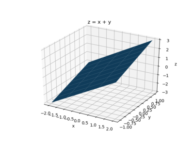
For example, to plot z=10+y over the ranges of x and y specified higher up - the code would be:

                        fig            =            plt            .            figure            (            num            =            1            ,            clear            =            True            )            ax            =            fig            .            add_subplot            (            1            ,            one            ,            one            ,            projection            =            '3d'            )            (            10            ,            y            )            =            np            .            meshgrid            (            np            .            arange            (            -            ii            ,            two.1            ,            1            ),            np            .            arange            (            -            1            ,            1.1            ,            .            25            ))            z            =            ten            +            y            ax            .            plot_surface            (            ten            ,            y            ,            z            )            ax            .            set            (            xlabel            =            'ten'            ,            ylabel            =            'y'            ,            zlabel            =            'z'            ,            title            =            'z = ten + y'            )            fig            .            tight_layout            ()          

and the graph is:

SurfExp01 py.png

If you want to make it more colorful, you tin import colormaps and and so use one; here is the consummate code:

                        import            numpy            every bit            np            from            mpl_toolkits.mplot3d            import            axes3d            import            matplotlib.pyplot            as            plt            from            matplotlib            import            cm            fig            =            plt            .            figure            (            num            =            ane            ,            clear            =            True            )            ax            =            fig            .            add_subplot            (            ane            ,            1            ,            ane            ,            projection            =            '3d'            )            (            x            ,            y            )            =            np            .            meshgrid            (            np            .            arange            (            -            2            ,            ii.1            ,            1            ),            np            .            arange            (            -            1            ,            1.ane            ,            .            25            ))            z            =            10            +            y            ax            .            plot_surface            (            x            ,            y            ,            z            ,            cmap            =            cm            .            copper            )            ax            .            set            (            xlabel            =            '10'            ,            ylabel            =            'y'            ,            zlabel            =            'z'            ,            title            =            'z = x + y'            )            fig            .            tight_layout            ()          

SurfExp01c py.png

To run across all the colormaps, afterward importing the cm group merely type

help(cm)        

to see the names or go to Colormap Reference to see the colors.


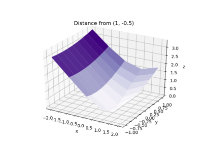
To find the distance r from a particular point, say (1,-0.five), y'all just demand to modify the function. Since the distance between two points \((x, y)\) and \((x_0, y_0)\) is given by \( r=\sqrt{(10-x_0)^2+(y-y_0)^two} \) the code could be:

                        fig            =            plt            .            figure            (            num            =            one            ,            articulate            =            True            )            ax            =            fig            .            add_subplot            (            ane            ,            1            ,            one            ,            projection            =            '3d'            )            (            x            ,            y            )            =            np            .            meshgrid            (            np            .            arange            (            -            2            ,            2.one            ,            ane            ),            np            .            arange            (            -            1            ,            one.1            ,            .            25            ))            z            =            np            .            sqrt            ((            x            -            (            1            ))            **            two            +            (            y            -            (            -            0.five            ))            **            two            )            ax            .            plot_surface            (            ten            ,            y            ,            z            ,            cmap            =            cm            .            Purples            )            ax            .            set            (            xlabel            =            'x'            ,            ylabel            =            'y'            ,            zlabel            =            'z'            ,            title            =            'Distance from (1, -0.5)'            )            fig            .            tight_layout            ()          

and the plot is

SurfExp02c py.png

Examples Using Refined Grids

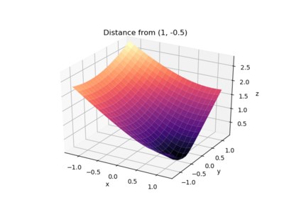
You lot can also utilize a effectively grid to brand a better-looking plot:

                        fig            =            plt            .            figure            (            num            =            one            ,            clear            =            True            )            ax            =            fig            .            add_subplot            (            1            ,            1            ,            1            ,            projection            =            '3d'            )            (            x            ,            y            )            =            np            .            meshgrid            (            np            .            linspace            (            -            one.ii            ,            1.2            ,            20            ),            np            .            linspace            (            -            ane.2            ,            1.2            ,            20            ))            z            =            np            .            sqrt            ((            x            -            (            1            ))            **            ii            +            (            y            -            (            -            0.5            ))            **            two            )            ax            .            plot_surface            (            10            ,            y            ,            z            ,            cmap            =            cm            .            magma            )            ax            .            fix            (            xlabel            =            '10'            ,            ylabel            =            'y'            ,            zlabel            =            'z'            ,            title            =            'Distance from (1, -0.5)'            )            fig            .            tight_layout            ()          

and the plot is:

SurfExp03c py.png

Using Other Coordinate Systems

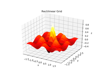
The plotting commands such as plot_surface and plot_wireframe generate surfaces based on matrices of x, y, and z coordinates, respectively, but y'all can also use other coordinate systems to calculate where the points get. Equally an case, the part

\( z = east^{-\sqrt{x^2+y^2}}~\cos(4x)~\cos(4y) \)

could be plotted on a rectilinear grid using:

                        fig            =            plt            .            figure            (            num            =            1            ,            clear            =            True            )            ax            =            fig            .            add_subplot            (            1            ,            1            ,            ane            ,            projection            =            '3d'            )            (            x            ,            y            )            =            np            .            meshgrid            (            np            .            linspace            (            -            one.8            ,            1.8            ,            41            ),            np            .            linspace            (            -            1.viii            ,            ane.8            ,            41            ))            z            =            np            .            exp            (            -            np            .            sqrt            (            10            **            2            +            y            **            2            ))            *            np            .            cos            (            4            *            x            )            *            np            .            cos            (            four            *            y            )            ax            .            plot_surface            (            10            ,            y            ,            z            ,            cmap            =            cm            .            hot            )            ax            .            ready            (            xlabel            =            'x'            ,            ylabel            =            'y'            ,            zlabel            =            'z'            ,            title            =            'Rectilinear Grid'            )            fig            .            tight_layout            ()          

giving

SurfChip01 py.png

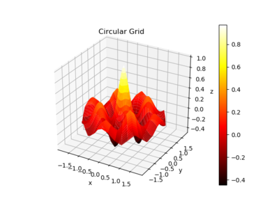
It could likewise exist plotted on a circular domain using polar coordinates. To exercise that, r and \(\theta\) coordinates could be generated using meshgrid and the appropriate x, y, and z values could exist obtained by noting that \(x=r\cos(\theta)\) and \(y=r\sin(\theta)\). z can then exist calculated from any combination of x, y, r, and \(\theta\):

                        fig            =            plt            .            figure            (            num            =            1            ,            clear            =            True            )            ax            =            fig            .            add_subplot            (            1            ,            1            ,            ane            ,            projection            =            '3d'            )            (            r            ,            theta            )            =            np            .            meshgrid            (            np            .            linspace            (            0            ,            1.8            ,            41            ),            np            .            linspace            (            0            ,            two            *            np            .            pi            ,            41            ))            ten            =            r            *            np            .            cos            (            theta            )            y            =            r            *            np            .            sin            (            theta            )            z            =            np            .            exp            (            -            r            )            *            np            .            cos            (            four            *            x            )            *            np            .            cos            (            4            *            y            )            ax            .            plot_surface            (            ten            ,            y            ,            z            ,            cmap            =            cm            .            hot            )            ax            .            set up            (            xlabel            =            'ten'            ,            ylabel            =            'y'            ,            zlabel            =            'z'            ,            title            =            'Circular Filigree'            )            fig            .            tight_layout            ()          

produces:

SurfChip01c py.png

Color Bars

You may desire to add a color bar to indicate the values assigned to particular colors. This may be done using the colorbar() command just to utilize information technology you need to have access to a variable that refers to your surface plot - annotation how the variable chipplot is used below:

                        fig            =            plt            .            figure            (            num            =            1            ,            clear            =            True            )            ax            =            fig            .            add_subplot            (            1            ,            1            ,            ane            ,            projection            =            '3d'            )            (            r            ,            theta            )            =            np            .            meshgrid            (            np            .            linspace            (            0            ,            1.8            ,            41            ),            np            .            linspace            (            0            ,            2            *            np            .            pi            ,            41            ))            x            =            r            *            np            .            cos            (            theta            )            y            =            r            *            np            .            sin            (            theta            )            z            =            np            .            exp            (            -            r            )            *            np            .            cos            (            4            *            ten            )            *            np            .            cos            (            iv            *            y            )            chipplot            =            ax            .            plot_surface            (            x            ,            y            ,            z            ,            cmap            =            cm            .            hot            )            ax            .            set            (            xlabel            =            'x'            ,            ylabel            =            'y'            ,            zlabel            =            'z'            ,            title            =            'Round Grid'            )            fig            .            colorbar            (            chipplot            )            fig            .            tight_layout            ()          

produces

SurfChip01cb py.png

There Is No Effort

                        import            numpy            as            np            from            mpl_toolkits.mplot3d            import            axes3d            import            matplotlib.pyplot            as            plt            from            matplotlib            import            cm            fig            =            plt            .            figure            (            num            =            1            ,            clear            =            True            )            ax            =            fig            .            add_subplot            (            1            ,            one            ,            1            ,            projection            =            '3d'            )            (            theta            ,            phi            )            =            np            .            meshgrid            (            np            .            linspace            (            0            ,            2            *            np            .            pi            ,            41            ),            np            .            linspace            (            0            ,            two            *            np            .            pi            ,            41            ))            ten            =            (            3            +            np            .            cos            (            phi            ))            *            np            .            cos            (            theta            )            y            =            (            3            +            np            .            cos            (            phi            ))            *            np            .            sin            (            theta            )            z            =            np            .            sin            (            phi            )            def            fun            (            t            ,            f            ):            return            (            np            .            cos            (            f            +            ii            *            t            )            +            1            )            /            2            dplot            =            ax            .            plot_surface            (            ten            ,            y            ,            z            ,            facecolors            =            cm            .            jet            (            fun            (            theta            ,            phi            )))            ax            .            set up            (            xlabel            =            'x'            ,            ylabel            =            'y'            ,            zlabel            =            'z'            ,            xlim            =            [            -            4            ,            four            ],            ylim            =            [            -            4            ,            4            ],            zlim            =            [            -            iv            ,            iv            ],            xticks            =            [            -            4            ,            -            two            ,            ii            ,            4            ],            yticks            =            [            -            four            ,            -            2            ,            two            ,            4            ],            zticks            =            [            -            1            ,            0            ,            1            ],            title            =            'Donut!'            )            fig            .            tight_layout            ()            fig            .            savefig            (            'Donut_py.png'            )          
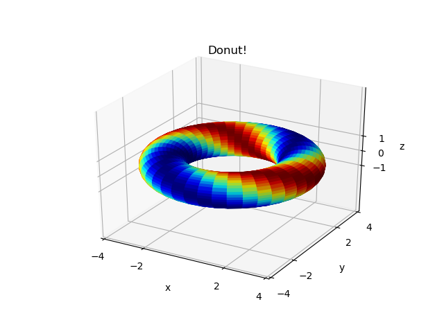
Donut py.png

Questions

Mail service your questions by editing the give-and-take page of this commodity. Edit the page, then curl to the bottom and add a question by putting in the characters *{{Q}}, followed by your question and finally your signature (with four tildes, i.due east. ~~~~). Using the {{Q}} will automatically put the page in the category of pages with questions - other editors hoping to assist out can and then go to that category page to see where the questions are. See the page for Template:Q for details and examples.

External Links

References

ramosopirted.blogspot.com

Source: https://pundit.pratt.duke.edu/wiki/Python:Plotting_Surfaces

0 Response to "how to draw plane in 3d plot python"

Post a Comment

Iklan Atas Artikel

Iklan Tengah Artikel 1

Iklan Tengah Artikel 2

Iklan Bawah Artikel